11 Biodiversity: Richness, Diversity, & Evenness
Data Type: Tabular Data (within eco_indicators)
Spatial Scope: Maritimes
Duration 1970-2022
Source: Bundy et al. 2017
11.1 Introduction to Indicator
The eco_indicators dataset provides several metrics of biodiversity from trawl surveys in the Canadian Atlantic, representing three subattributes of biodiversity (Bundy, Gomez, and Cook 2017).
- Species Richness
- Species Richness: Number of species recorded in a given year and sampling area.
- Margalef’s Species Richness: A richness index that standardizes species count by sample size.
- Species Diversity
- Shannon Diversity: Entropy-based measure of diversity that accounts for both species richness and the relative abundances of species in a given year and sampling area.
- Hill Diversity (N1): Exponential of the Shannon index; effective number of species in a sample, accounting for both species richness and evenness.
- Species Evenness
- Pielou Evenness: Measure of how evenly individuals are distributed among species.
- Hill Dominance (N2): Reciprocal of Simpson’s index; effective indication of the number of common species in a sample.
- Heips Evenness Index: Evenness metric derived from Shannon diversity that scales between 0 and 1 and expresses how close a community is to having equal abundances across species.
11.2 View Data
library(tidyr)
library(plotly)
library(stringr)

plotly_df <- data@data %>% inner_join(global_cols3)

# function to create plot with dropdown menu ------------------------------
make_biomass_dropdown_plot <- function(df,
                                      year_col   = "year",
                                      region_col = "region",
                                      value_suffix = "_value") {

  # convert to long format
  long <- df %>%
    janitor::clean_names() %>%
    pivot_longer(
      cols = ends_with(value_suffix),
      names_to = "metric",
      values_to = "value"
    ) %>%
    # remove suffix
    mutate(
      metric = str_remove(metric, "_value")
    ) %>%
    # drop NAs (some regions don't have data for some variables or years)
    tidyr::drop_na(value)

  # find all metrics and regions
  metrics <- unique(long$metric)
  regions <- unique(long[[region_col]])

  # clean names for dropdown panels, helper
  pretty_label <- function(x) str_to_title(gsub("_", " ", x)) %>% gsub("Lb","L B",.) %>% gsub("Mb","M B",.)

  # build plot -----------------
  p <- plot_ly()

  # add line traces
  for (metric_i in seq_along(metrics)) {
    m <- metrics[metric_i]

    for (region_i in regions) {
      dat <- long %>%
        filter(metric == m, .data[[region_col]] == region_i)

      group_name <- unique(dat$region_group)
      color <- unique(dat$color)
      linetype <- unique(dat$linetype)
      width <- unique(dat$linewidth)

      # If a region truly has no data for that metric, add an empty trace
      # (keeps trace indexing stable)
      if (nrow(dat) == 0) {
        dat <- tibble::tibble(!!year_col := integer(0), value = numeric(0))
      }

      p <- p %>% add_lines(
        data = dat,
        x = ~.data[[year_col]],
        y = ~value,
        name = as.character(region_i),
        legendgroup = group_name,
        legendgrouptitle = list(
          text = ifelse(group_name == "ESS",
                        "Eastern Scotian Shelf Zones",
                        "Western Scotian Shelf Zones"
          )),
        showlegend = (metric_i == 1),
        visible = (metric_i == 1),
        line = list(color = color, dash = linetype),
        hovertemplate = paste0("<b>", region_i,":</b> ","%{y:.3f}<extra></extra>")      )

    }
  }

  n_regions <- length(regions)
  n_traces  <- length(metrics) * n_regions

  buttons <- lapply(seq_along(metrics), function(metric_i) {
    vis <- rep(FALSE, n_traces)
    shl <- rep(FALSE, n_traces)

    idx_start <- (metric_i - 1) * n_regions + 1
    idx_end   <- metric_i * n_regions
    vis[idx_start:idx_end] <- TRUE
    shl[idx_start:idx_end] <- TRUE

    list(
      method = "update",
      args = list(
        list(visible = vis, showlegend = shl),
        list(
          title = pretty_label(metrics[metric_i]),
          yaxis = list(title =  pretty_label(metrics[metric_i]))
        )
      ),
      label = pretty_label(metrics[metric_i])
    )
  })

  p %>%
    layout(
      barmode = "stack",
      hovermode = "x unified",
      title = pretty_label(metrics[1]),
      xaxis = list(title = str_to_title(year_col)),  # keep one bar per year
      yaxis = list(title = metrics[1], fixedrange = TRUE),
      legend = list(
        x = 1.02, xanchor = "left",
        y = 1,    yanchor = "top",
        groupclick = "toggleitem",
        itemdoubleclick = FALSE
      ),
      updatemenus = list(list(
        type = "dropdown",
        x = -.1, xanchor = "left",
        y = 1.15, yanchor = "top",
        buttons = buttons
      )),
      margin = list(r = 180, t = 80)
    )
}

# usage:
p <- make_biomass_dropdown_plot(plotly_df)
p <- p %>% config(displayModeBar= F)

p
Figure 11.1: Biodiversity Indicators in all NAFO regions and Scotian Shelf regions overall. Use dropdown menu to select indicator, and click legend to toggle regions.
11.3 Summary and Trends
Trend and summary values are automatically generated; data were last updated on marea package install on 2026-02-10
Biodiversity variables show considerable variation between management areas (ESS, WSS) and NAFO divisions (4V, 4W, 4X), sometimes with non-linear patterns across the sampling span (Fig. 11.1).
Although not all variables can be simply interpreted by directional trends, biodiversity trends in the Eastern Scotian Shelf are generally decreasing and biodiversity trends in the Western Scotian Shelf are generally increasing.
Across the sampling span, the Eastern Scotian Shelf experienced increases in 2 variables (2 significant), and decreases in 5 variables (5 significant). The Western Scotian Shelf experienced increases in 6 variables (6 significant), and decreases in 1 variable (0 significant) (Fig. 11.2).
When split by category, biodiversity trends become more clear (Fig. 11.2).
- Species Richness: Both indicators of species richness (Species Richness and Margalef Species Richness Index) increased significantly since the 1970s in the ESS and WSS.
- Species Diversity: Indicators for diversity (Shannon Diversity and Hill’s Diversity-N1) followed similar trends: Increases in the WSS and decreases in the ESS over time.
- Species Evenness: For two of three indicators of evenness (Hill’s Dominance-N2, and Peilou Evenness), evenness increased in the WSS and decreased in the ESS. For the third indicator of evenness (Heip’s Evenness), evenness decreased in the ESS, and had a non-significant decreasing trend in the WSS.
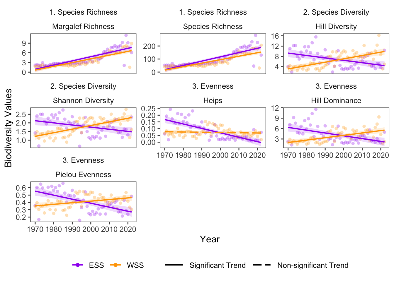
Figure 11.2: Biodiversity Variable trends for ESS and WSS
11.3.1 Summary Table by NAFO Region and Biodiversity Variable
Trends of each Biodiversity variable for each NAFO region within the Eastern and Western Scotian Shelf (1970-2022) are shown below (Table 11.1).
| variable | Eastern Scotian Shelf biodiversity Trends | Western Scotian Shelf biodiversity Trends |
|---|---|---|
| Heips |
4VN: -1.90e-03 ∗ 4VS: -2.86e-03 ∗ 4W: -3.87e-03 ∗ ESS: -3.27e-03 ∗ |
4X: -1.89e-04 WSS: -1.89e-04 |
| Hill Diversity |
4VN: 1.17e-01 ∗ 4VS: -6.68e-02 ∗ 4W: -7.01e-02 ∗ ESS: -1.03e-01 ∗ |
4X: 1.31e-01 ∗ WSS: 1.31e-01 ∗ |
| Hill Dominance |
4VN: 5.27e-02 ∗ 4VS: -4.47e-02 ∗ 4W: -7.24e-02 ∗ ESS: -8.51e-02 ∗ |
4X: 6.86e-02 ∗ WSS: 6.86e-02 ∗ |
| Margalef Richness |
4VN: 9.34e-02 ∗ 4VS: 8.94e-02 ∗ 4W: 9.60e-02 ∗ ESS: 1.15e-01 ∗ |
4X: 1.16e-01 ∗ WSS: 1.16e-01 ∗ |
| Pielou Evenness |
4VN: 1.43e-04 4VS: -6.00e-03 ∗ 4W: -5.15e-03 ∗ ESS: -6.03e-03 ∗ |
4X: 2.18e-03 ∗ WSS: 2.18e-03 ∗ |
| Shannon Diversity |
4VN: 1.72e-02 ∗ 4VS: -1.51e-02 ∗ 4W: -9.26e-03 ∗ ESS: -1.54e-02 ∗ |
4X: 2.09e-02 ∗ WSS: 2.09e-02 ∗ |
| Species Richness |
4VN: 2.10e+00 ∗ 4VS: 2.27e+00 ∗ 4W: 2.33e+00 ∗ ESS: 2.91e+00 ∗ |
4X: 2.67e+00 ∗ WSS: 2.67e+00 ∗ |
11.4 Relevance to Research and Stock Assessments
Biodiversity metrics such as species richness, diversity, and evenness capture complementary aspects of community structure; namely, the number of species present and how evenly biomass or abundance is distributed among them. In Atlantic Canada, these indices are used to track community-level changes alongside species-level trends, and integrated into marine spatial planning (Ward-Paige and Bundy 2016).
Biodiversity metrics can be strongly influenced by Anthropogenic effects to ecosystems. For example, the cod collapse in Atlantic Canada in the 1980s led to restructuring of marine fish communities which was detectable by changes in biodiversity indicators (McCain et al. 2016). Spatial patterns in these indicators can also be used in conservation management, for example, by targeting areas of high biodiversity for the implementation of protected or conserved areas (Shackell and Frank 2003).
Because each of these biodiversity metrics are calculated by species identification in surveys, trends can also be driven by changes in data collection method or improved species identification.
11.5 Variable Definitions
| variable | description | unit |
|---|---|---|
| year | Year of data collection | |
| region | Region over which observations are summarized | |
| SpeciesRichness_ALL_value | Species richness in samples | Number of species |
| ShannonDiversity_ALL_value | Shannon Diversity | Dimensionless |
| MargalefRichness_ALL_value | Margalef Richness Index | Dimensionless |
| PielouEvenness_ALL_value | Pielou Evenness Index | Dimensionless |
| HillDiversity_ALL_value | Hill Diversity (N1) | Effective number of species |
| HillDominance_ALL_value | Hill Dominance (N2) | Effective number of dominant/very abundant species |
| Heips_ALL_value | Heips evenness index | Dimensionless |