12 Structure & Function: Top of the Food Web
Data Type: Tabular Data (within eco_indicators)
Spatial Scope: Maritimes
Duration 1970-2022
Source: Bundy et al. 2017
12.1 Introduction to Indicator
The eco_indicators dataset provides indicators of ecosystem structure with focus on the top of the food web (Bundy, Gomez, and Cook 2017).
- Large Fish Indicator: Proportion of large fish (>35cm) in the community.
- Proportion of Predators: Proportion of predatory fish (feeding on fish or non-planktonic invertebrates).
These indicators provide data on how the marine community is structured, and have relevance to top-down controls on the ecosystem.
12.2 View Data
library(tidyr)
library(plotly)
library(stringr)

plotly_df <- data@data %>% inner_join(global_cols3)

# function to create plot with dropdown menu ------------------------------
make_topfoodweb_dropdown_plot <- function(df,
                                      year_col   = "year",
                                      region_col = "region",
                                      value_suffix = "_value") {

  # convert to long format
  long <- df %>%
    janitor::clean_names() %>%
    pivot_longer(
      cols = ends_with(value_suffix),
      names_to = "metric",
      values_to = "value"
    ) %>%
    # remove suffix
    mutate(
      metric = str_remove(metric, "_value")
    ) %>%
    # drop NAs (some regions don't have data for some variables or years)
    tidyr::drop_na(value)

  # find all metrics and regions
  metrics <- unique(long$metric)
  regions <- unique(long[[region_col]])

  # assign regions to consistent colors
 # region_colors <- setNames(hcl.colors(length(regions), palette = "Dark 3"), regions)

  # clean names for dropdown panels, helper
  pretty_label <- function(x) str_to_title(gsub("_", " ", x))

  # build plot -----------------
  p <- plot_ly()

  # Add bar traces: metric1 has region1..K, metric2 has region1..K, ...
  for (metric_i in seq_along(metrics)) {
    m <- metrics[metric_i]

    for (region_i in regions) {
      dat <- long %>%
        filter(metric == m, .data[[region_col]] == region_i) %>%
        group_by(.data[[year_col]],color, linetype, linewidth, region_group, region_group_label) %>%     # in case you have multiple rows per year
        summarise(value = sum(value), .groups = "drop") %>%
        arrange(.data[[year_col]])

      group_name <- unique(dat$region_group)
      color <- unique(dat$color)
      linetype <- unique(dat$linetype)
      width <- unique(dat$linewidth)

      # If a region truly has no data for that metric, add an empty trace
      # (keeps trace indexing stable)
      if (nrow(dat) == 0) {
        dat <- tibble::tibble(!!year_col := integer(0), value = numeric(0))
      }

      p <- p %>% add_lines(
        data = dat,
        x = ~.data[[year_col]],
        y = ~value,
        name = as.character(region_i),
        legendgroup = group_name,
        legendgrouptitle = list(
          text =
            ifelse(group_name == "ESS",
                   "Eastern Scotian Shelf Zones",
                   "Western Scotian Shelf Zones"
                    )),
        showlegend = (metric_i == 1),
        visible = (metric_i == 1),
        line = list(color = color, dash = linetype),
        hovertemplate = paste0("<b>", region_i,":</b> ","%{y:.3f}<extra></extra>")      )

    }
  }

  n_regions <- length(regions)
  n_traces  <- length(metrics) * n_regions

  buttons <- lapply(seq_along(metrics), function(metric_i) {
    vis <- rep(FALSE, n_traces)
    shl <- rep(FALSE, n_traces)

    idx_start <- (metric_i - 1) * n_regions + 1
    idx_end   <- metric_i * n_regions
    vis[idx_start:idx_end] <- TRUE
    shl[idx_start:idx_end] <- TRUE

    list(
      method = "update",
      args = list(
        list(visible = vis, showlegend = shl),
        list(
          title = pretty_label(metrics[metric_i]),
          yaxis = list(title =  pretty_label(metrics[metric_i]))
        )
      ),
      label = pretty_label(metrics[metric_i])
    )
  })

  p %>%
    layout(
      barmode = "stack",
      hovermode = "x unified",
      title = pretty_label(metrics[1]),
      xaxis = list(title = str_to_title(year_col)),  # keep one bar per year
      yaxis = list(title = pretty_label(metrics[1]), fixedrange = TRUE),
      legend = list(
        x = 1.02, xanchor = "left",
        y = 1,    yanchor = "top",
        groupclick = "toggleitem",
        itemdoubleclick = FALSE
      ),
      updatemenus = list(list(
        type = "dropdown",
        x = -.1, xanchor = "left",
        y = 1.15, yanchor = "top",
        buttons = buttons
      )),
      margin = list(r = 180, t = 80)
    )
}

# usage:
p <- make_topfoodweb_dropdown_plot(plotly_df)
p <- p %>% config(displayModeBar= F)

p
Figure 12.1: Top of the food web indicators in all NAFO divisions and Scotian Shelf regions overall. Use dropdown menu to select indicator, and click legend to toggle regions.
12.3 Summary and Trends
Trend and summary values are automatically generated; data were last updated on marea package install on 2026-02-10
Top of the food web variables are changing across the Scotian Shelf region with noisy trends through time (Fig. 12.1).
The proportion of top of the food web species is decreasing in the Eastern Scotian Shelf with 2 variables showing negative trends through time (2 significant). In the Western Scotian Shelf, the proportion of large fish has decreased significantly through time, but the proportion of predators has increased (Fig. 12.2).
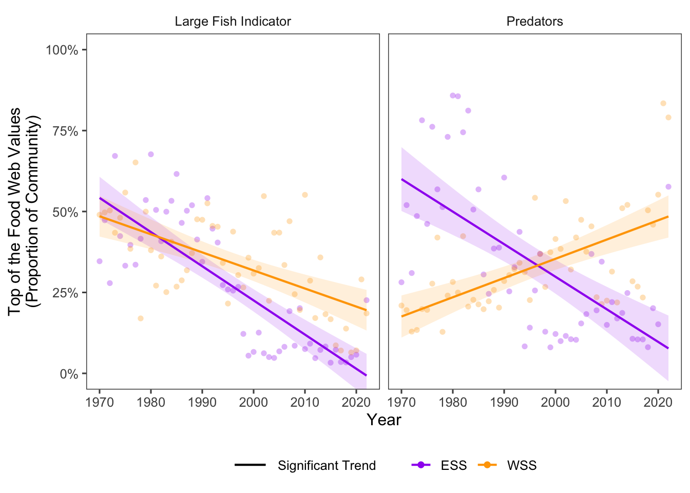
Figure 12.2: Top of the Food Web trends for ESS and WSS
12.3.1 Summary Table by NAFO Region and Top of the Food Web Variable
Trends of each top of the food web variable for each NAFO region within the Eastern and Western Scotian Shelf (1970-2022) are shown below (Table 12.1).
| variable | Eastern Scotian Shelf Trends | Western Scotian Shelf Trends |
|---|---|---|
| Large Fish Indicator Value |
4VN: -1.40e-02 ∗ 4VS: -9.86e-03 ∗ 4W: -8.70e-03 ∗ ESS: -1.06e-02 ∗ |
4X: -5.58e-03 ∗ WSS: -5.58e-03 ∗ |
| Predators |
4VN: -7.68e-03 ∗ 4VS: -1.38e-02 ∗ 4W: -9.61e-03 ∗ ESS: -1.02e-02 ∗ |
4X: 5.94e-03 ∗ WSS: 5.94e-03 ∗ |
12.4 Relevance to Research and Stock Assessments
Fishing activities disproportionately target large fish and predator species, so top of the food web indicators are expected to respond to fishing activities in exploited systems.
In Atlantic Canada, removal of predator species via fishing activity can lead to trophic cascades, affecting marine ecosystems through top-down change (Frank et al. 2005). Declines of large-bodied predator species can result in “fishing down the food web” strategies in marine fisheries, which might result in a phase of increased landings or revenue from lower-trophic level species, but ultimately unsustainability for the marine ecosystem (Pauly et al. 1998).
12.5 Variable Definitions
| variable | description | unit |
|---|---|---|
| year | Year of trawl survey | |
| region | Region over which values are summarized | |
| LargeFishIndicator_value | Proportion of fish >35cm | Proportion |
| PREDATORS_ALL_value | Proportion of predators | Proportion |