16 Structure & Function: Fish Community Condition
Data Type: Tabular Data (within eco_indicators)
Spatial Scope: Maritimes
Duration 1970-2022
Source: Bundy et al. 2017
16.1 Introduction to Indicator
Fulton’s Condition factor (TW 1904) is a ratio of body weight to length, or the relative “plumpness” of fish. Fulton’s condition is calculated as condition = 100 * weight / length^3, and is used for a proximal for fish health. Higher condition factors represent fish that are heavier at a given length, and are assumed to be in better condition. However, Fulton’s condition does not always correlate with more precise measures of fish body condition, especially when the assumption of isometric growth is violated.
While comparisons of Fulton’s condition between species or subgroups might be hindered by inherent differences in mass to length ratios between group, comparisons of Fulton’s condition can be made between individuals within a species or in aggregate for a species over time to capture overall trends or indicate resource limitations or excesses (Ricker 1975). Fulton’s condition can also change seasonally, representing variation in nutritional resources available throughout the year in seasonal environments.
Here, condition is presented at the community level. Fulton’s Community Condition index is calculated from the abundance (A) weighted mean weight (W) at length (L) by species (j) from information in the survey as:
\[ \frac{\sum_{j=1}^{l} (K_j \cdot A_j)} {\sum_{j=1}^{l} A_j} \]
where
\[ K_j = \frac{W_j}{L_j^3} \times 100 \]
16.2 View Data
library(tidyr)
library(plotly)
library(stringr)

plotly_df <- data@data %>% inner_join(global_cols3)

# function to create plot with dropdown menu ------------------------------
make_biomass_dropdown_plot <- function(df,
                                      year_col   = "year",
                                      region_col = "region",
                                      value_suffix = "_value") {

  # convert to long format
  long <- df %>%
    janitor::clean_names() %>%
    pivot_longer(
      cols = ends_with(value_suffix),
      names_to = "metric",
      values_to = "value"
    ) %>%
    # remove suffix
    mutate(
      metric = str_remove(metric, "_value")
    ) %>%
    # drop NAs (some regions don't have data for some variables or years)
    tidyr::drop_na(value)

  # find all metrics and regions
  metrics <- unique(long$metric)
  regions <- unique(long[[region_col]])

  # clean names for dropdown panels, helper
  pretty_label <- function(x) str_to_title(gsub("_", " ", x)) %>% gsub("Lb","Large B",.) %>% gsub("Mb","Medium B",.) %>% str_replace("C Condition ","")

  # build plot -----------------
  p <- plot_ly()

 # add line traces
  for (metric_i in seq_along(metrics)) {
    m <- metrics[metric_i]

    for (region_i in regions) {
      dat <- long %>%
        filter(metric == m, .data[[region_col]] == region_i)

      group_name <- unique(dat$region_group)
      color <- unique(dat$color)
      linetype <- unique(dat$linetype)
      width <- unique(dat$linewidth)

      # If a region truly has no data for that metric, add an empty trace
      # (keeps trace indexing stable)
      if (nrow(dat) == 0) {
        dat <- tibble::tibble(!!year_col := integer(0), value = numeric(0))
      }

      p <- p %>% add_lines(
        data = dat,
        x = ~.data[[year_col]],
        y = ~value,
        name = as.character(region_i),
        legendgroup = group_name,
        legendgrouptitle = list(
          text = ifelse(group_name == "ESS",
                        "Eastern Scotian Shelf Zones",
                        "Western Scotian Shelf Zones"
          )),
        showlegend = (metric_i == 1),
        visible = (metric_i == 1),
        line = list(color = color, dash = linetype),
        hovertemplate = paste0("<b>", region_i,":</b> ","%{y:.3f}<extra></extra>")      )

    }
  }

  n_regions <- length(regions)
  n_traces  <- length(metrics) * n_regions

  buttons <- lapply(seq_along(metrics), function(metric_i) {
    vis <- rep(FALSE, n_traces)
    shl <- rep(FALSE, n_traces)

    idx_start <- (metric_i - 1) * n_regions + 1
    idx_end   <- metric_i * n_regions
    vis[idx_start:idx_end] <- TRUE
    shl[idx_start:idx_end] <- TRUE

    list(
      method = "update",
      args = list(
        list(visible = vis, showlegend = shl),
        list(
          title = pretty_label(metrics[metric_i]),
          yaxis = list(title = "Community Condition")
        )
      ),
      label = pretty_label(metrics[metric_i])
    )
  })

  p %>%
    layout(
      barmode = "stack",
      hovermode = "x unified",
      title = pretty_label(metrics[1]),
      xaxis = list(title = str_to_title(year_col)),  # keep one bar per year
      yaxis = list(title = "Community Condition", fixedrange = TRUE),
      legend = list(
        x = 1.02, xanchor = "left",
        y = 1,    yanchor = "top",
        groupclick = "toggleitem",
        itemdoubleclick = FALSE
      ),
      updatemenus = list(list(
        type = "dropdown",
        x = -.1, xanchor = "left",
        y = 1.15, yanchor = "top",
        buttons = buttons
      )),
      margin = list(r = 180, t = 80),
            # add horizontal line at 1
      shapes = list(
        type = "line",
        xref = "paper",
        yref = "y",
        x0 = 0,
        x1 = 1,
        y0 = 1,
        y1 = 1,
        line = list(color = "black", width = 2, dash = "dash")
      )
    )
}

# usage:
p <- make_biomass_dropdown_plot(plotly_df)
p <- p %>% config(displayModeBar= F)

p
Figure 16.1: Community condition in all NAFO regions and Scotian Shelf regions overall.
16.3 Summary and Trends
Trend and summary values are automatically generated; data were last updated on marea package install on 2026-02-10
Community condition changes through time have differed between regions, with more pronounced negative change observed on the Eastern Scotian Shelf (Fig. 16.1). Across the 6 functional groups, condition in the Eastern Scotian Shelf decreased, and community condition in the Western Scotian Shelf mostly decreased. In the Eastern Scotian Shelf, all groups had decreasing trends (4 significant), some non-linear (eg finfish). In the Western Scotian Shelf, 2 groups increased in condition through time (0 significant), and 4 groups decreased in condition over time (2) (Fig. 16.2).
Community condition changes through time have differed between regions, with more pronounced negative changes observed on the Eastern Scotian Shelf (Fig. 16.1. Across 6 functional groups, condition in the Eastern Scotian Shelf decreased, and community condition in the Western Scotian Shelf mostly decreased. In the Eastern Scotian Shelf, 5 groups decreased over time(4 significant), and 1 group increased (0 significant), with some nonlinearities observed (e.g., finfish). In the Western Scotian Shelf, 2 groups increased in condition through time (0 significant), and 4 groups decreased in condition over time (2) (Fig. 16.2).
The strongest decrease in condition was in the Finfish group in the ESS region (Fig. 16.2), and the strongest increase in condition was in the Piscivore group in the ESS region (Fig. 16.2).
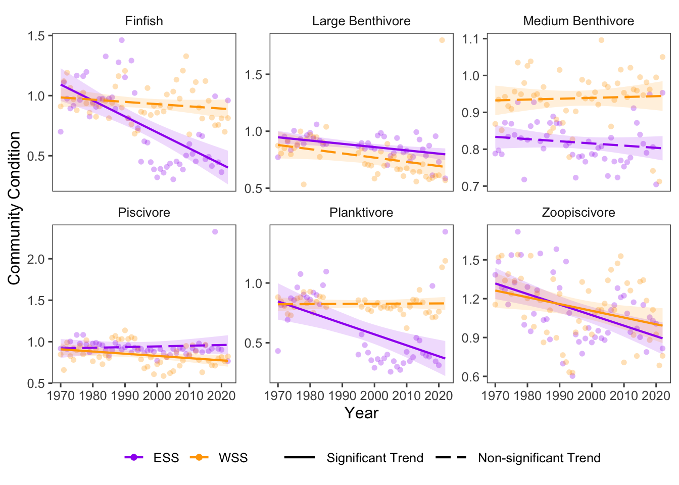
Figure 16.2: Fulton’s Condition for fish groups over time in Scotian Shelf
16.3.1 Summary Table by NAFO Region and Functional Group
Trends in Community Condition for each functional group in each NAFO region within the Eastern and Western Scotian Shelf (1970-2022) region are shown in the table below (Table 16.1).
| variable | Eastern Scotian Shelf ccondition Trends | Western Scotian Shelf ccondition Trends |
|---|---|---|
| Finfish |
4VN: -2.97e-03 4VS: -1.73e-02 ∗ 4W: -8.13e-03 ∗ ESS: -1.41e-02 ∗ |
4X: -1.85e-03 WSS: -1.85e-03 |
| Large Benthivore |
4W: -5.46e-03 ∗ ESS: 1.30e-03 |
4X: -3.95e-03 ∗ WSS: -1.77e-04 |
| Medium Benthivore |
4VN: -1.45e-03 4VS: -2.69e-03 ∗ 4W: -1.99e-04 ESS: -2.21e-03 |
4X: 2.29e-04 WSS: 2.29e-04 |
| Piscivore |
4VN: -5.06e-04 4VS: -1.82e-03 ∗ 4W: 9.59e-04 ESS: -1.11e-03 |
4X: -2.67e-03 ∗ WSS: -2.67e-03 ∗ |
| Planktivore |
4W: -4.75e-03 ∗ ESS: -7.00e-03 ∗ |
4X: 7.58e-05 WSS: 3.73e-03 |
| Zoopiscivore |
4VN: -2.11e-03 4VS: -5.09e-03 ∗ 4W: -9.79e-03 ∗ ESS: -9.97e-03 ∗ |
4X: -5.22e-03 ∗ WSS: -5.22e-03 ∗ |
16.4 Relevance to Research and Stock Assessments
Fulton’s condition at the scale of fish stocks reveals several insights into stock health. For cod, stocks with higher Fulton’s condition factors have higher recruitment potential, and higher biological management reference points for safe exploitation without collapse (Fmed) (Rätz and Lloret 2003).
16.5 Variable Definitions
| Variable | Description | Unit |
|---|---|---|
| year | Year of trawl surveys | |
| region | Region over which data are summarized | |
| CCondition_{taxon}_value | Fulton’s Condition Index | 100*Weight/Length3 |