26 Fishing Pressure: Distribution of Fishing Pressure
Data Type: Tabular Data (within eco_indicators)
Spatial Scope: Maritimes
Duration 1970-2022
Source: Bundy et al. 2017
26.1 Introduction to Indicator
The distribution of fishing pressure is characterized by three proximal indicators.
- Diversity of Target Species: the number of species targeted by commercial fisheries; proximal variable for fisheries effort.
- Mean Trophic Level of Fisheries Landings: the trophic position of harvested fish.
- Marine Trophic Index of Fisheries Landings: tropic average of landed fish, normally with a cutoff (here, 3.5) to capture change in fisheries effort in high-trophic-level species.
26.2 View Data
library(tidyr)
library(plotly)
library(stringr)

plotly_df <- data@data %>% inner_join(global_cols3)

# function to create plot with dropdown menu ------------------------------
make_distFP_dropdown_plot <- function(df,
                                      year_col   = "year",
                                      region_col = "region",
                                      value_suffix = "_value") {

  # convert to long format
  long <- df %>%
    janitor::clean_names() %>%
    pivot_longer(
      cols = ends_with(value_suffix),
      names_to = "metric",
      values_to = "value"
    ) %>%
    # remove suffix
    mutate(
      metric = str_remove(metric, "_value")
    ) %>%
    # drop NAs (some regions don't have data for some variables or years)
    tidyr::drop_na(value)

  # find all metrics and regions
  metrics <- sort(unique(long$metric))
  regions <- unique(long[[region_col]])

  # clean names for dropdown panels, helper
  pretty_label <- function(x) str_replace(x, "diversity_target_spp_all","Diversity of Target Species") %>%
    str_replace(.,"mean_tl_landings", "Mean TL of Landings") %>% str_replace(.,"mti_landings_3_25","MTI of Landings")

  # build plot -----------------
  p <- plot_ly()

  # Add bar traces: metric1 has region1..K, metric2 has region1..K, ...
  for (metric_i in seq_along(metrics)) {
    m <- metrics[metric_i]

    for (region_i in regions) {
      dat <- long %>%
        filter(metric == m, .data[[region_col]] == region_i)

      group_name <- unique(dat$region_group)
      color <- unique(dat$color)
      linetype <- unique(dat$linetype)
      width <- unique(dat$linewidth)

      # If a region truly has no data for that metric, add an empty trace
      # (keeps trace indexing stable)
      if (nrow(dat) == 0) {
        dat <- tibble::tibble(!!year_col := integer(0), value = numeric(0))
      }

      p <- p %>% add_lines(
        data = dat,
        x = ~.data[[year_col]],
        y = ~value,
        name = as.character(region_i),
        legendgroup = group_name,
        legendgrouptitle = list(
          text = ifelse(group_name == "ESS",
                        "Eastern Scotian Shelf Zones",
                        "Western Scotian Shelf Zones"
          )),
        showlegend = (metric_i == 1),
        visible = (metric_i == 1),
        line = list(color = color, dash = linetype),
        hovertemplate = paste0("<b>", region_i,":</b> ","%{y:.3f}<extra></extra>")      )

    }
  }

  n_regions <- length(regions)
  n_traces  <- length(metrics) * n_regions

  buttons <- lapply(seq_along(metrics), function(metric_i) {
    vis <- rep(FALSE, n_traces)
    shl <- rep(FALSE, n_traces)

    idx_start <- (metric_i - 1) * n_regions + 1
    idx_end   <- metric_i * n_regions
    vis[idx_start:idx_end] <- TRUE
    shl[idx_start:idx_end] <- TRUE

    list(
      method = "update",
      args = list(
        list(visible = vis, showlegend = shl),
        list(
          title = pretty_label(metrics[metric_i]),
          yaxis = list(title =pretty_label(metrics[metric_i]))
        )
      ),
      label = pretty_label(metrics[metric_i])
    )
  })

  p %>%
    layout(
      barmode = "stack",
      hovermode = "x unified",
      title = pretty_label(metrics[1]),
      xaxis = list(title = str_to_title(year_col)),  # keep one bar per year
      yaxis = list(title = pretty_label(metrics[1]), fixedrange = TRUE),
      legend = list(
        x = 1.02, xanchor = "left",
        y = 1,    yanchor = "top",
        groupclick = "toggleitem",
        itemdoubleclick = FALSE
      ),
      updatemenus = list(list(
        type = "dropdown",
        x = -.1, xanchor = "left",
        y = 1.15, yanchor = "top",
        buttons = buttons
      )),
      margin = list(r = 180, t = 80)
    )
}

# usage:
p <- make_distFP_dropdown_plot(plotly_df)
p <- p %>% config(displayModeBar= F)

p
Figure 26.1: Distribution of Fishing Pressure Variables in Scotian Shelf regions; 1970-2022. Use dropdown box to select a target trophic level, and click legend to toggle regions.
26.3 Summary and Trends
Trend and summary values are automatically generated; data were last updated on marea package install on 2026-02-10
Although trends between NAFO zones varied over time (Fig. 26.1), overall trends in the Eastern and Western Scotian Shelf regions were mostly consistent (Fig. 26.2).
In both regions:
- Diversity of Target Species increased
- Mean Trophic Level of Landings significantly decreased
- Marine Trophic Index of Landings decreased, but with a non-significant trend for ESS.
The increase in diversity of target species indicates a growing distribution of fishing pressure throughout the marine community. Decreases in Mean TL and MTI of landings indicate that harvest activities have shifted away from high trophic level species, although this could be due to previous overharvesting of species at high trophic levels.
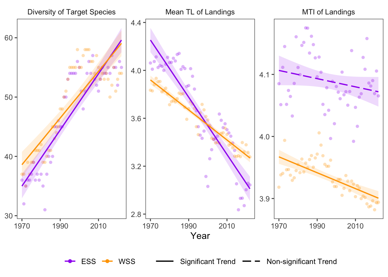
Figure 26.2: Trends in distribution of fishing pressure variables over time in the Eastern and Western Scotian Shelf regions.
26.3.1 Summary Table by Region and Functional Group
Trends in distribution of fishing pressure variables for each NAFO region within the Eastern and Western Scotian Shelf (1970-2022) are shown in the table below (Table 26.1).
| Variable | Eastern Scotian Shelf Trends | Western Scotian Shelf Trends |
|---|---|---|
| Diversity of Target Species |
4VN: 5.49e-02 4VS: 1.82e-01 ∗ 4W: 4.87e-01 ∗ ESS: 4.73e-01 ∗ |
4X: 3.93e-01 ∗ WSS: 3.93e-01 ∗ |
| MTI of Landings |
4VN: -1.21e-04 4VS: -9.64e-04 4W: -2.16e-04 ESS: -6.61e-04 |
4X: -1.28e-03 ∗ WSS: -1.28e-03 ∗ |
| Mean TL of Landings |
4VN: -2.22e-02 ∗ 4VS: -3.57e-02 ∗ 4W: -1.31e-02 ∗ ESS: -2.39e-02 ∗ |
4X: -1.25e-02 ∗ WSS: -1.25e-02 ∗ |
26.4 Relevance to Research and Stock Assessments
Increases in the diversity of target species represent expansions of fisheries effort across the marine community (Bundy, Gomez, and Cook 2017). Expansions of fishing effort across the community could be a result of decreased abundance of historically targeted species.
Decreases in mean trophic level and Marine Trophic Index oflandings represent shifts from fisheries efforts targeted towards high trophic level species towards species lower in the food chain. These shifts are consistent with the “fishing down the food web” process, where the depletion of large predatory fish has resulted in fishieries expansions towards lower trophic level groups (Pauly et al. 1998).
26.5 Variable Definitions
| variable | description | unit |
|---|---|---|
| year | Year of data collection | |
| region | Region over which data are summarized | |
| DiversityTargetSpp_ALL_value | Number of species targeted by commercial fishing | Number of Species |
| MeanTL.Landings_value | Mean Trophic Level of landings | Trophic Level |
| MTI.Landings_3.25_value | Marine Trophic Index of landings | Trophic Level |