25 Fishing Pressure: Fished Groups
Data Type: Tabular Data (within eco_indicators)
Spatial Scope: Maritimes
Duration 1970-2022
Source: Bundy et al. 2017
25.1 Introduction to Indicator
Fishing pressure is a relative metric of intensity of exploitation on fished groups. Here, fishing pressure is presented per guild and calculated as a ratio: fishing pressure = total biomass / total landings (Bundy, Gomez, and Cook 2017).
Since fishing pressure is calculated as a ratio, changes in fishing pressure can either result from changes to total landings, changes to total biomass, or both. Conversely, stability in fishing pressure does not guarantee that total landings and total biomass are also stable; if each value changes in the same direction, fishing pressure might remain stable.
This indicator focuses on the fishing pressure on fished groups: Clupeids, Flatfish, Forage Fish, Gadoids, Groundfish, and Skates.
25.2 View Data
library(tidyr)
library(plotly)
library(stringr)

plotly_df <- data@data %>% inner_join(global_cols3)

# function to create plot with dropdown menu ------------------------------
make_biomass_dropdown_plot <- function(df,
                                      year_col   = "year",
                                      region_col = "region",
                                      value_suffix = "_value") {

  # convert to long format
  long <- df %>%
    janitor::clean_names() %>%
    pivot_longer(
      cols = ends_with(value_suffix),
      names_to = "metric",
      values_to = "value"
    ) %>%
    # remove suffix
    mutate(
      metric = str_remove(metric, "_value")
    ) %>%
    # drop NAs (some regions don't have data for some variables or years)
    tidyr::drop_na(value)

  # find all metrics and regions
  metrics <- unique(long$metric)
  regions <- unique(long[[region_col]])

  # clean names for dropdown panels, helper
  pretty_label <- function(x) str_to_title(gsub("fp_", "", x))

  # build plot -----------------
  p <- plot_ly()

  # add line traces
  for (metric_i in seq_along(metrics)) {
    m <- metrics[metric_i]

    for (region_i in regions) {
      dat <- long %>%
        filter(metric == m, .data[[region_col]] == region_i)

      group_name <- unique(dat$region_group)
      color <- unique(dat$color)
      linetype <- unique(dat$linetype)
      width <- unique(dat$linewidth)

      # If a region truly has no data for that metric, add an empty trace
      # (keeps trace indexing stable)
      if (nrow(dat) == 0) {
        dat <- tibble::tibble(!!year_col := integer(0), value = numeric(0))
      }

      p <- p %>% add_lines(
        data = dat,
        x = ~.data[[year_col]],
        y = ~value,
        name = as.character(region_i),
        legendgroup = group_name,
        legendgrouptitle = list(
          text = ifelse(group_name == "ESS",
                        "Eastern Scotian Shelf Zones",
                        "Western Scotian Shelf Zones"
          )),
        showlegend = (metric_i == 1),
        visible = (metric_i == 1),
        line = list(color = color, dash = linetype),
        hovertemplate = paste0("<b>", region_i,":</b> ","%{y:.3f}<extra></extra>")      )

    }
  }

  n_regions <- length(regions)
  n_traces  <- length(metrics) * n_regions

  buttons <- lapply(seq_along(metrics), function(metric_i) {
    vis <- rep(FALSE, n_traces)
    shl <- rep(FALSE, n_traces)

    idx_start <- (metric_i - 1) * n_regions + 1
    idx_end   <- metric_i * n_regions
    vis[idx_start:idx_end] <- TRUE
    shl[idx_start:idx_end] <- TRUE

    list(
      method = "update",
      args = list(
        list(visible = vis, showlegend = shl),
        list(
          title = pretty_label(metrics[metric_i]),
          yaxis = list(title = "Fishing Pressure")
        )
      ),
      label = pretty_label(metrics[metric_i])
    )
  })

  p %>%
    layout(
      barmode = "stack",
      hovermode = "x unified",
      title = pretty_label(metrics[1]),
      xaxis = list(title = str_to_title(year_col)),  # keep one bar per year
      yaxis = list(title = "Fishing Pressure", fixedrange = TRUE),
      legend = list(
        x = 1.02, xanchor = "left",
        y = 1,    yanchor = "top",
        groupclick = "toggleitem",
        itemdoubleclick = FALSE
      ),
      updatemenus = list(list(
        type = "dropdown",
        x = 0, xanchor = "left",
        y = 1.15, yanchor = "top",
        buttons = buttons
      )),
      margin = list(r = 180, t = 80),
            # add horizontal line at 1
      shapes = list(
        type = "line",
        xref = "paper",
        yref = "y",
        x0 = 0,
        x1 = 1,
        y0 = 1,
        y1 = 1,
        line = list(color = "black", width = 2, dash = "dash")
      )
    )
}

# usage:
p <- make_biomass_dropdown_plot(plotly_df)
p <- p %>% config(displayModeBar= F)

p
Figure 25.1: Fishing pressure in all NAFO regions and Scotian Shelf regions over time; 1970-2022.
25.3 Summary and Trends
Trend and summary values are automatically generated; data were last updated on marea package install on 2026-02-10
Estimates of fishing pressure are highly variable across time and between regions, and often exceed theoretical bounds (upper limit of 1), likely due to inaccurate estimates of total biomass (Fig. 25.1). Still, interpreting trends can reveal some insights into changes in fishing pressure to Scotian Shelf communities.
When fitting linear models to fishing pressure on fished groups over time (1970-2022) , some regional trends emerge. In the Eastern Scotian Shelf, 1 group experienced increasing fishing pressure (0 significant), and 5 groups experienced decreasing fishing pressure (5 significant). In the Western Scotian Shelf, 3 groups experienced increasing fishing pressure (0 significant) and 3 groups experienced decreasing fishing pressure (3 significant).
The strongest increase in fishing pressure was on the Forage group in the WSS region, and the strongest decrease was on the Clupeids group in the ESS region (Fig. 25.2).
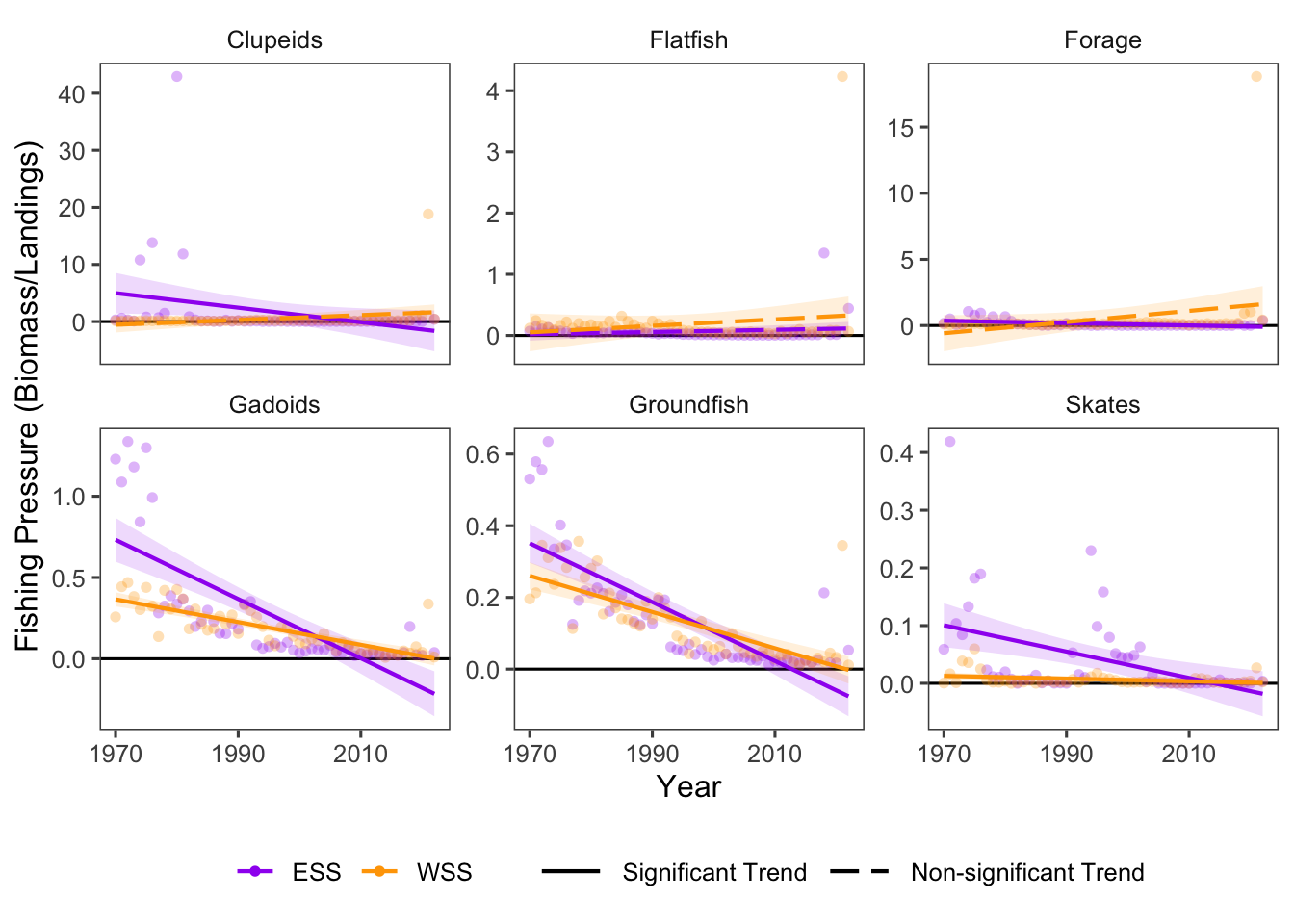
Figure 25.2: Fishing Pressure for guilds over time in Scotian Shelf.
25.3.1 Summary Table by Region and Guild
Trends of Fishing Pressure over time for each guild and NAFO region within the Eastern and Western Scotian Shelf (1970-2022) are shown in the table below (Table 25.1).
| taxon | Eastern Scotian Shelf | Western Scotian Shelf |
|---|---|---|
| Clupeids |
4VN: -1.07e-01 ∗ 4VS: -2.22e-02 ∗ 4W: -7.05e-02 ∗ ESS: -1.19e-01 ∗ |
4X: 4.22e-02 WSS: 4.22e-02 |
| Flatfish |
4VN: -5.36e-03 ∗ 4VS: -1.50e-03 ∗ 4W: 1.75e-04 ESS: 1.58e-03 |
4X: 5.32e-03 WSS: 5.32e-03 |
| Forage |
4VN: -3.76e-01 4VS: -3.11e-02 4W: -2.22e-02 ∗ ESS: -8.71e-03 ∗ |
4X: 4.23e-02 WSS: 4.23e-02 |
| Gadoids |
4VN: -2.95e-02 ∗ 4VS: -1.69e-02 ∗ 4W: -1.96e-02 ∗ ESS: -1.78e-02 ∗ |
4X: -6.99e-03 ∗ WSS: -6.99e-03 ∗ |
| Groundfish |
4VN: -1.49e-02 ∗ 4VS: -5.23e-03 ∗ 4W: -1.05e-02 ∗ ESS: -8.07e-03 ∗ |
4X: -5.05e-03 ∗ WSS: -5.05e-03 ∗ |
| Skates |
4VN: -5.19e-04 ∗ 4VS: -6.96e-04 4W: -5.53e-03 ∗ ESS: -2.25e-03 ∗ |
4X: -2.35e-04 ∗ WSS: -2.35e-04 ∗ |
25.4 Relevance to Research and Stock Assessments
Fishing pressure affects populations both by direct removal of individuals from the population, and by alteration of the size-structure and demographic properties of populations. Fishing pressure generally targets larger, older fish, thus truncating the age of the remaining population by removing mature and fecund individuals (Tu, Chen, and Hsieh 2018). High fishing pressure can contribute to the decline or collapse of exploited fisheries (Pinsky and Byler 2015; Essington et al. 2015).
25.5 Variable Definitions
| variable | description | unit |
|---|---|---|
| year | Year of data collection | |
| region | Area over which observations are summarized | |
| FP_{TAXON}_value | Fishing Pressure, calculated as Biomass/Landings | Proportion |