27 Commercial Fisheries
Data Type: Tabular Data (within eco_indicators)
Spatial Scope: Maritimes
Duration 1970-2022
Source: Bundy et al. 2017
27.1 Introduction to Indicator
Commercial fishing is a major marine human activity in Atlantic Canada, with several high-value species present in the region. Fisheries landing data can indicate the pressure exerted on target groups, the pressure on communities, the trophic or ecosystem distributions of fishing pressure, and fisheries productivity. Landings can also indicate the pressure exerted on other species in the community via human disturbance, bycatch, and changes to species interactions.
Landings indicators are presented both as total landings in the community (Landings All), and landings per fished group (Bundy, Gomez, and Cook 2017).
27.2 View Data
library(tidyr)
library(plotly)
library(stringr)

plotly_df <- data@data %>% inner_join(global_cols2)

# function to create plot with dropdown menu ------------------------------
make_biomass_dropdown_plot <- function(df,
                                      year_col   = "year",
                                      region_col = "region",
                                      value_suffix = "_value") {

  # convert to long format
  long <- df %>%
    janitor::clean_names() %>%
    pivot_longer(
      cols = ends_with(value_suffix),
      names_to = "metric",
      values_to = "value"
    ) %>%
    # remove suffix
    mutate(
      metric = str_remove(metric, "_value")
    ) %>%
    # drop NAs (some regions don't have data for some variables or years)
    tidyr::drop_na(value)

  # find all metrics and regions
  metrics <- unique(long$metric)
  regions <- unique(long[[region_col]])


  # clean names for dropdown panels, helper
  pretty_label <- function(x) str_to_title(gsub("_", " ", x)) %>% gsub(" L$","",.)

  # build plot -----------------
  p <- plot_ly()

  # Add bar traces: metric1 has region1..K, metric2 has region1..K, ...
  for (metric_i in seq_along(metrics)) {
    m <- metrics[metric_i]

    for (region_i in regions) {
      dat <- long %>%
        filter(metric == m, .data[[region_col]] == region_i) %>%
        group_by(.data[[year_col]],color, region_group, region_group_label) %>%     # in case you have multiple rows per year
        summarise(value = sum(value), .groups = "drop") %>%
        arrange(.data[[year_col]])

        group_name <- unique(dat$region_group)
        color <- unique(dat$color)

      # If a region truly has no data for that metric, add an empty trace
      # (keeps trace indexing stable)
      if (nrow(dat) == 0) {
        dat <- tibble::tibble(!!year_col := integer(0), value = numeric(0))
      }

        p <- p %>% add_bars(
          data = dat,
          x = ~.data[[year_col]],
          y = ~value,
          name = as.character(region_i),
          legendgroup = group_name,
          legendgrouptitle = list(
            text =  ifelse(group_name == "ESS",
                           "Eastern Scotian Shelf Zones",
                           "Western Scotian Shelf Zones")),
          showlegend = (metric_i == 1),
          visible = (metric_i == 1),
          marker = list(color = color),
          hovertemplate = paste0("<b>", region_i,":</b> ","%{y:,.2s}<extra></extra>")      )
    }
  }

  n_regions <- length(regions)
  n_traces  <- length(metrics) * n_regions

  buttons <- lapply(seq_along(metrics), function(metric_i) {
    vis <- rep(FALSE, n_traces)
    shl <- rep(FALSE, n_traces)

    idx_start <- (metric_i - 1) * n_regions + 1
    idx_end   <- metric_i * n_regions
    vis[idx_start:idx_end] <- TRUE
    shl[idx_start:idx_end] <- TRUE

    list(
      method = "update",
      args = list(
        list(visible = vis, showlegend = shl),
        list(
          title = pretty_label(metrics[metric_i]),
          yaxis = list(title = paste0(pretty_label(metrics[metric_i])," (tonnes)"))
        )
      ),
      label = pretty_label(metrics[metric_i])
    )
  })

  p %>%
    layout(
      barmode = "stack",
      hovermode = "x unified",
      title = pretty_label(metrics[1]),
      xaxis = list(title = str_to_title(year_col), type = "category"),  # keep one bar per year
      yaxis = list(title = paste0(pretty_label(metrics[1])," (tonnes)"), fixedrange = TRUE),
      legend = list(
        x = 1.02, xanchor = "left",
        y = 1,    yanchor = "top",
        groupclick = "toggleitem",
        itemdoubleclick = FALSE
      ),
      updatemenus = list(list(
        type = "dropdown",
        x = 0, xanchor = "left",
        y = 1.15, yanchor = "top",
        buttons = buttons
      )),
      margin = list(r = 180, t = 80)
    )
}

# usage:
p <- make_biomass_dropdown_plot(plotly_df)
p <- p %>% config(displayModeBar= F)

p
Figure 27.1: Commercial Fisheries Landings in Scotian Shelf regions; 1970-2022. Use dropdown box to select a target fishery, and click legend to isolate regions.
27.3 Summary and Trends
Trend and summary values are automatically generated; data were last updated on marea package install on 2026-02-10
While trends between management and NAFO regions have varied over time, landings in the Scotian Shelf have generally decreased since the 1970s (Fig. 27.1).
In the Eastern Scotian Shelf, landings for 8 of 10 groups decreased over the sampling span (8 significant), and 2 increased (2). In the Western Scotian Shelf, 9 groups decreased (8 significant), and 1 increased (1 significant) (Fig. 27.2).
The strongest decrease was observed in the Finfish group in the ESS region, and the strongest increase was in the Invertebrates in the WSS region (Fig. 27.2).
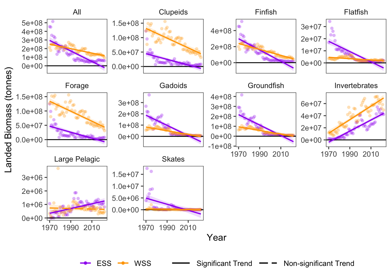
Figure 27.2: Overall slopes of landed values over time. Lines show linear model fits, and shadows represent 95% confidence intervals. Line color and dash pattern indicate region and significant trend (p < 0.05)
27.3.1 Summary Table by Region and Commercial Fishery
Trends over time for commercial fisheries landings in each NAFO region within the Eastern and Western Scotian Shelf (1970-2022) are shown in the table below (Table 27.1).
| taxon | Eastern Scotian Shelf Landings Trends (tonnes/year) | Western Scotian Shelf Landings Trends (tonnes/year) |
|---|---|---|
| All |
4VN: -1.12e+06 ∗ 4VS: -9.37e+05 ∗ 4W: -4.06e+06 ∗ ESS: -6.11e+06 ∗ |
4X: -2.58e+06 ∗ WSS: -2.58e+06 ∗ |
| Clupeids |
4VN: -2.25e+05 ∗ 4VS: -8.53e+04 ∗ 4W: -6.66e+05 ∗ ESS: -9.76e+05 ∗ |
4X: -1.69e+06 ∗ WSS: -1.69e+06 ∗ |
| Finfish |
4VN: -1.23e+06 ∗ 4VS: -1.45e+06 ∗ 4W: -4.34e+06 ∗ ESS: -7.02e+06 ∗ |
4X: -3.70e+06 ∗ WSS: -3.70e+06 ∗ |
| Flatfish |
4VN: -8.80e+04 ∗ 4VS: -1.94e+05 ∗ 4W: -1.41e+05 ∗ ESS: -4.23e+05 ∗ |
4X: -5.53e+04 ∗ WSS: -5.53e+04 ∗ |
| Forage |
4VN: -2.25e+05 ∗ 4VS: -9.53e+04 ∗ 4W: -7.23e+05 ∗ ESS: -1.04e+06 ∗ |
4X: -1.74e+06 ∗ WSS: -1.74e+06 ∗ |
| Gadoids |
4VN: -6.86e+05 ∗ 4VS: -9.55e+05 ∗ 4W: -2.87e+06 ∗ ESS: -4.52e+06 ∗ |
4X: -1.64e+06 ∗ WSS: -1.64e+06 ∗ |
| Groundfish |
4VN: -7.80e+05 ∗ 4VS: -1.19e+06 ∗ 4W: -3.27e+06 ∗ ESS: -5.23e+06 ∗ |
4X: -1.82e+06 ∗ WSS: -1.82e+06 ∗ |
| Invertebrates |
4VN: 1.10e+05 ∗ 4VS: 5.16e+05 ∗ 4W: 2.88e+05 ∗ ESS: 9.14e+05 ∗ |
4X: 1.12e+06 ∗ WSS: 1.12e+06 ∗ |
| Large Pelagic |
4VN: -3.38e+02 ∗ 4VS: 1.75e+03 4W: 1.62e+04 ∗ ESS: 1.76e+04 ∗ |
4X: -1.98e+03 WSS: -1.98e+03 |
| Skates |
4VN: -1.15e+03 ∗ 4VS: -1.88e+04 ∗ 4W: -1.09e+05 ∗ ESS: -1.29e+05 ∗ |
4X: -6.19e+03 ∗ WSS: -6.19e+03 ∗ |
27.4 Relevance to Research and Stock Assessments
Total landings can lend insight to the pressures on stocks and marine ecosystems.
High landings indicate that many individuals were removed from the system and non-target species may have faced pressures from disturbance in fishing processes.
Low landings, alternatively, might indicate the removal of fishing pressure (particularly when fisheries are closed), or could indicate reduced catch per unit effort in the active stocks.
27.5 Variable Definitions
| variable | description | unit |
|---|---|---|
| year | Year of data collection | |
| region | Region in which landings are summarized | |
landings_{taxon}_valueor landings_{taxon}.L_value
|
Biomass landed of selected taxa and region | (tonnes) |