7 Satellite Ocean Colour
Data Type: Gridded Data
Spatial Scope: Northwest Atlantic
Duration: 1998-2024
Source: SOPhyE group, DFO
Contact:
7.1 Introduction to Indicator
The Satellite Ocean Colour dataset is a product of the Satellite Ocean Color and Phytoplankton Ecology (SOPhyE) group at Bedford Institute of Oceanography. Satellite Ocean Colour data uses remotely sensed multispectral data capturing the reflectance properties of the ocean to proximally serve as an indicator of plankton biomass, chlorophyll, and productivity of marine environments. Given differences in absorption and reflectance between plankton species and non-algal particulates, multispecral ocean color measurements categorize the particulate content of water, and infer indators of algal abundnace, biomass, and productivity.
Here, satellite ocean color is used to infer five indicator variables across space:
- Start Day of spring phytoplankton bloom
- Duration of the spring phytoplankton bloom
- Maximum concentration during the spring phytoplankton bloom (amplitude)
- Total chlorophyll-a produced during the spring phytoplankton bloom (magnitude)
- Average chlorophyll-a produced annually
Each of these indicators are expected to respond to oceanographic variability and long-term climate change, with variable responses across space or between algal species At mid-latitudes, climate change is expected to delay the date of spring blooms at a global scale (Henson et al. 2018), and changes in other oceanographic variables such as stratification can affect bloom magnitude (Song et al. 2011).
7.2 View Data
# prepare sf shapes as coordinates
# NAFO regions
sf <- sf %>% st_transform(crs = terra::crs(t_duration))
# coastline
data("coastline")
# get timespan
timespan <- paste0(
  str_replace(years[1],"y.",""),
  "-",
  str_replace(years[length(years)],"y.","")
  )
# get bounding box
bbox <- ext(t_start[[1]])


# plot means over timespan ------------------
means_baseplot <- function(df){

  # find mean of every cell, excluding NAs
  mean_df <- app(df, "mean", na.rm=T)

  # base plot
  p <- ggplot() +
    geom_sf(data = coastline) +
    geom_spatraster(data = mean_df,aes(fill = mean)) +
    geom_sf(data = sf, aes(color = I(color)),
            fill = "transparent", linewidth = .5)+
    coord_sf(xlim = c(bbox$xmin, bbox$xmax),
             ylim = c(bbox$ymin, bbox$ymax), expand=F) +
    scale_fill_viridis_c(na.value = "transparent") +
    theme_light(base_size = 9) +
    theme(legend.position = "bottom",
          legend.title.position = "top",
          legend.key.height = unit(6,"pt"),
          legend.key.width = unit(24,"pt"))
   return(p)
}

## plot all mean values
mean_start_p <- means_baseplot(t_start) +
  scale_fill_viridis_c(breaks = c(60, 121),labels = c("Mar 1","May 1"),
                       na.value = "transparent") +
  labs(title = "Mean Bloom Start",
       subtitle = timespan,
       fill = "Day of Year")

mean_duration_p <- means_baseplot(t_duration) +
  labs(title = "Mean Bloom Duration",
       subtitle = timespan,
       fill = "Number of Days")

mean_amplitude_p <- means_baseplot(amplitude) +
  labs(title = "Mean Bloom Amplitude",
       subtitle = timespan,
       fill = "Max. Concentration (mg/m^3)")

mean_magnitude_p <- means_baseplot(magnitude) +
  labs(title = "Mean Bloom Magnitude",
       subtitle = timespan,
       fill = "Total Chlorophyll (mg/m^3)")

mean_mean_p <- means_baseplot(mean) +
  labs(title = "Mean Avg. Chl.",
       subtitle = timespan,
       fill = "Chlorophyll (mg/m^3)")


# second, slopes per cell
trends_baseplot <- function(df){

  # function to apply to extract slopes over time for every cell
  slope_fun <- function(x) {
    if (all(is.na(x))) return(NA)
    # exclude cells that are 50% or more NA
    if (sum(is.na(x)) > length(x)*.5) return(NA)
    lm(x ~ c(1:length(x)))$coefficients[2]
  }
  # find mean of every cell, excluding NAs
  slope_df <- app(df, slope_fun)
  names(slope_df) <- "trend"

  # base plot
  p <- ggplot() +
    geom_spatraster(data = slope_df,aes(fill = trend)) +
    geom_sf(data = coastline) +
    geom_sf(data = sf, aes(color = I(color)),
            fill = "transparent", linewidth = .5)+
    coord_sf(xlim = c(bbox$xmin, bbox$xmax),
             ylim = c(bbox$ymin, bbox$ymax), expand=F) +
    scale_fill_gradient2(low = "#A6611A", high = "#018571",
                         na.value = "grey75") +
    theme_light(base_size = 9) +
    theme(legend.position = "bottom",
          legend.title.position = "top",
          legend.key.height = unit(5,"pt"),
          legend.key.width = unit(20,"pt"))
   return(p)
}

## plot all slope values
trend_start_p <- trends_baseplot(t_start) +
  labs(title = "Change in Bloom Start",
       subtitle = timespan,
       fill = "Days/Year")

trend_duration_p <- trends_baseplot(t_duration) +
  labs(title = "Change in Bloom Duration",
       subtitle = timespan,
       fill = "Number of Days/Year")

trend_amplitude_p <- trends_baseplot(amplitude) +
  labs(title = "Change in Amplitude",
       subtitle = timespan,
       fill = "Concentration/Year")

trend_magnitude_p <- trends_baseplot(magnitude) +
  labs(title = "Change in Magnitude",
       subtitle = timespan,
       fill = "Total Chlorophyll/Year")

trend_mean_p <- trends_baseplot(mean) +
  labs(title = "Change in Avg. Chl.",
       subtitle = timespan,
       fill = "Concentration Change/Year")


library(patchwork)
full_p <-
  (
    ((mean_start_p | mean_duration_p | mean_amplitude_p | mean_magnitude_p |mean_mean_p )  +
       plot_layout(axes = "collect") &
       theme(axis.text = element_blank(),
             legend.margin = margin(t = -4))
     )/
      (
        (trend_start_p | trend_duration_p | trend_amplitude_p | trend_magnitude_p |trend_mean_p ) +
          plot_layout(axes = "collect") &
          theme(axis.text = element_blank(),
                legend.margin = margin(t = -4))
        )
    )

full_p #+ ggview::canvas(10,7)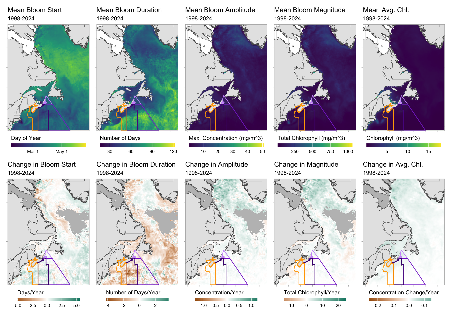
Figure 7.1: Summary values for Satellite Ocean Colour across space within the study region (Northwest Atlantic); 1998-2024. Top row shows mean values per raster cell of five ocean colour indicators. Bottom row shows slope values for variable values across time using linear models, with cells that contain 50% or more NA values excluded and shown in grey. Target NAFO regions for this report are shown in purple and orange. Note that many variables/year combinations have NA values, so more precise filtering may be required for more in-depth analyses.
7.3 Summary and Trends
Trend and summary values are automatically generated; data were last updated on marea package install on 2026-02-10
All Satellite Ocean Colour variables were variable across space, particularly between the inner and outer Scotian Shelf regions (Fig. 7.1). Within the target Scotian Shelf NAFO Divisions, space-averaged values for all indicators were more similar.
Within the NAFO divisions in the Eastern and Western Scotian Shelf:
- Mean bloom start date across years ranged from Mar 09 in division 4W to Mar 16 in division 4Vn.
- Mean bloom duration ranged from 49.24 days in division 4Vn to 79.83 days in division 4Vs.
- Mean bloom amplitude per cell ranged from 2.13 mg/m3; in division 4Vs to 5.8 mg/m3 in division 4Vn.
- Mean bloom magnitude per cell ranged from 38.24 days * mg/m3; in division 4Vs to 104.67 days * mg/m3 in division 4Vn.
- Mean average annual chlorophyll ranged from 0.34 mg/m3; in division 4Vs to 1.51 mg/m3 in division 4Vn.
Across time, spatially-averaged values for each metric within NAFO regions varied from year to year (Fig. 7.2). The general trends for each variable were as follows:
- Bloom start date shifted later in the year for 4 regions (2 significant), and shifted earlier for 0 regions (0 significant).
- Bloom became longer for 0 regions (0 significant), and became shorter for 4 regions (2 significant).
- Bloom amplitude increased for 4 regions (0 significant), and decreased for 0 regions (0 significant).
- Bloom magnitude increased for 4 regions (0 significant), and decreased for 0 regions (0 significant).
- Mean annual chlorophyll increased for 4 regions (4 significant), and decreased for 0 regions (0 significant).
Figure 7.2: Spatially-averaged values for satellite ocean colour indicators within NAFO regions in the Eastern and Western Scotian Shelf; 1998-2024.
7.3.1 Summary Table by Region
Linear trend summaries for each variable in each NAFO region can be found below (Table 7.1).
| variable | Eastern Scotian Shelf Trends | Western Scotian Shelf Trends |
|---|---|---|
| Bloom Start Day |
4Vn: 0.16 ± 0.7 4Vs: 0.15 ± 0.43 4W: 0.56 ± 0.38 ∗ |
4X: 0.43 ± 0.4 ∗ |
| Bloom Duration |
4Vn: -0.38 ± 0.59 4Vs: -0.26 ± 0.43 4W: -0.99 ± 0.47 ∗ |
4X: -0.82 ± 0.49 ∗ |
| Bloom Amplitude |
4Vn: 0.02 ± 0.09 4Vs: 0.02 ± 0.02 4W: 0 ± 0.03 |
4X: 0.02 ± 0.04 |
| Bloom Magnitude |
4Vn: 0.02 ± 0.09 4Vs: 0.02 ± 0.02 4W: 0 ± 0.03 |
4X: 0.02 ± 0.04 |
| Mean Chlorophyll |
4Vn: 0.02 ± 0.01 ∗ 4Vs: 0 ± 0 ∗ 4W: 0.01 ± 0 ∗ |
4X: 0.01 ± 0.01 ∗ |
7.4 Relevance to Research and Stock Assessments
Phytoplankton form the base of the marine food web, so bloom dynamics are directly relevant to fisheries and marine ecosystems through bottom-up effects. Changes in algal bloom dynamics can cause “mismatches” in timing between consumers (e.g., marine larvae) and algal nutrient sources (Platt, Fuentes-Yaco, and Frank 2003), and bloom activity can also include algal species that are harmful to ecosystems or humans (Boivin-Rioux et al. 2022).
In Atlantic Canada, spring bloom timing anomalies are predictive of larval fish survival, where earlier blooms result in greater survival of key harvested fish species (Platt, Fuentes-Yaco, and Frank 2003).
7.5 Variable Definitions
Satellite Ocean Colour is stored as a stars object in marea, with five data attributes arranged over three dimensions (x, y, time). See attribute names and definitions in the table below (Table 7.2)
| attribute | description | unit |
|---|---|---|
| t_start_value | Bloom start date | Day of year |
| t_duration_value | Bloom duration | Days |
| amplitude_real_value | Maximum concentration during the spring phytoplankton bloom period | mg/m3 |
| magnitude_real_value | Total chlorophyll-a produced during the spring phytoplankton bloom period | days*mg/m3 |
| annual_mean_value | Average chlorophyll-a over the year | mg/m3 |